↑
Datametri Logo
01
Heterogeneity and Sub-Group Analyses (Subgroup Forest Plot)
Random-Effects Subgroup Analysis
▼
"Isolate the Source of Methodological Contradictions"

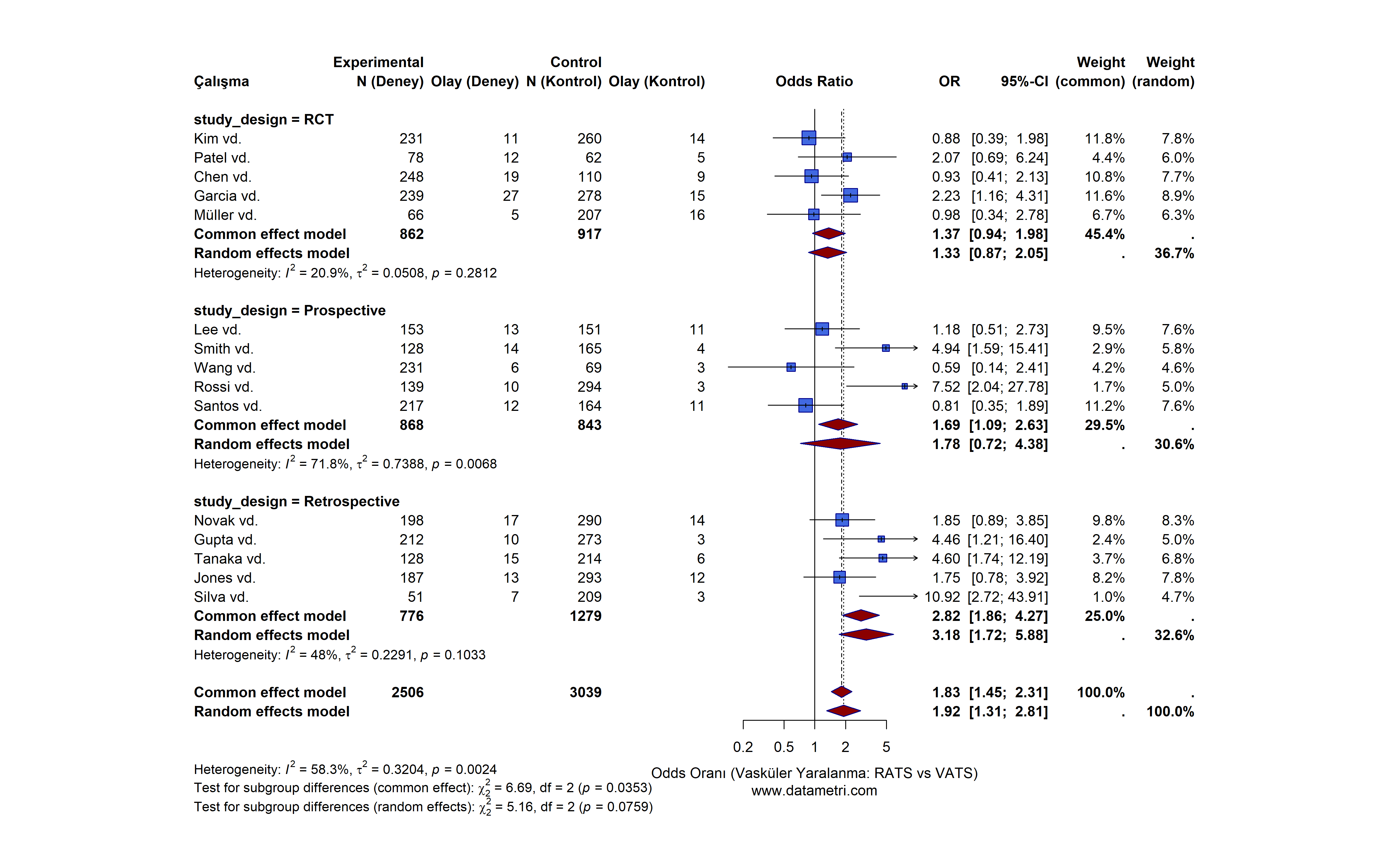
When calculating the overall effect of conflicting studies or studies conducted on different populations, we do not ignore methodological differences. We stratify studies based on predetermined categorical moderators (e.g., study design).

Which Questions Does This Analysis Answer?
  • When independent studies are statistically synthesized, what is the overall net direction of the effect?
  • Do the selected sub-groups (e.g., study design, applied dose, clinical stage) create a significant difference (heterogeneity) on the effectiveness of the intervention?
Added Value to Your Research

Resolves the problem of "inconsistency" in the literature. Mathematically isolates the source of differences without falling into the "comparing apples and oranges" fallacy frequently criticized by reviewers.
Sub-Group Analysis Forest Plot
This Forest Plot synthesizes the effect sizes (Odds Ratio - OR) and 95% Confidence Intervals of the studies via a Random-Effects Model. The analysis stratifies the studies according to "Study Design". The dark red diamonds indicate the pooled net effect size.
02
Publication Bias Audit (Contour-Enhanced Funnel Plot)
Trim and Fill Egger's Test
▼
"Reflect the Shadow of Unpublished Literature Onto Your Model"

The tendency for only statistically significant (p < .05) results to be published in the literature is the greatest methodological vulnerability of meta-analyses. We overcome this "file drawer problem" using advanced diagnostics.

Which Questions Does This Analysis Answer?
  • Is there a systematic publication bias present in the selected literature network?
  • If unpublished negative/insignificant studies were also present in the literature, in what direction and by how much would the pooled effect size we calculated change?
Added Value to Your Research

Proves that the meta-analysis findings are not the result of a biased literature review. High-impact factor (Q1) journals will not review any meta-analysis where publication bias has not been tested and adjusted.

Contour-Enhanced Funnel Plot
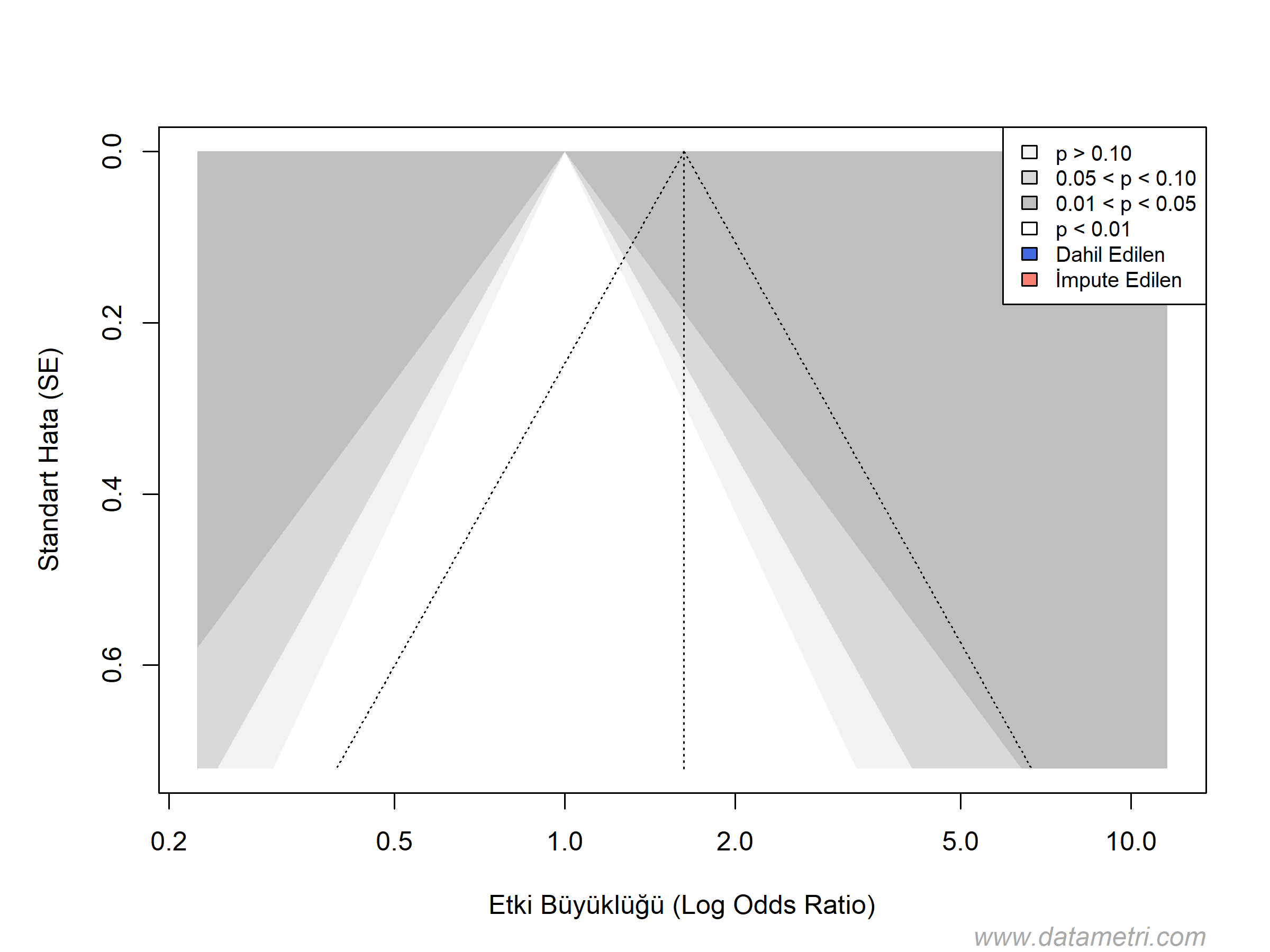
This Contour-Enhanced Funnel Plot is a publication bias audit combined with Egger's Regression Test. The blue dots represent published studies, while the salmon-colored triangles represent the "missing" studies simulated by the Trim and Fill algorithm and imputed into the model.
03
Outlier and Influence Diagnostics (Baujat Plot)
Leave-One-Out Outlier Detection
▼
"Statistically Expose Studies Disrupting the Overall Equilibrium"

In cases of high heterogeneity (I² > 50%), we do not perform random exclusions to determine which study disrupts the equilibrium of the overall model; instead, we apply algorithmic influence analyses.

Which Questions Does This Analysis Answer?
  • Which specific studies manipulate the direction of the overall outcome (pooled estimate)?
  • How does the overall effect change when studies that are the source of excessively high heterogeneity are removed (Leave-One-Out analysis)?
Added Value to Your Research

Equips the researcher with the power and scientific justification to state "it was proven to be statistically anomalous" rather than saying "it didn't fit my narrative" when excluding a study from the literature.

Baujat Diagnostic Plot
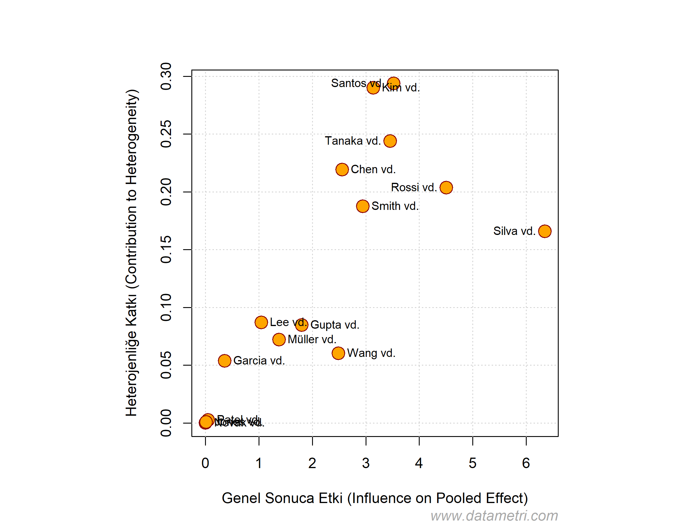
The Baujat Diagnostic Plot shows the position of each study within the meta-analysis ecosystem. The horizontal axis determines the study's deviating influence on the overall result; the vertical axis determines its contribution to heterogeneity. The orange points moving away to the upper right quadrant (outliers) threaten the model's reliability.
04
Meta-Regression and Cumulative Meta-Analysis Models
Meta-Regression Cumulative Forest
▼
"Model the Literature as a Dynamic Process"

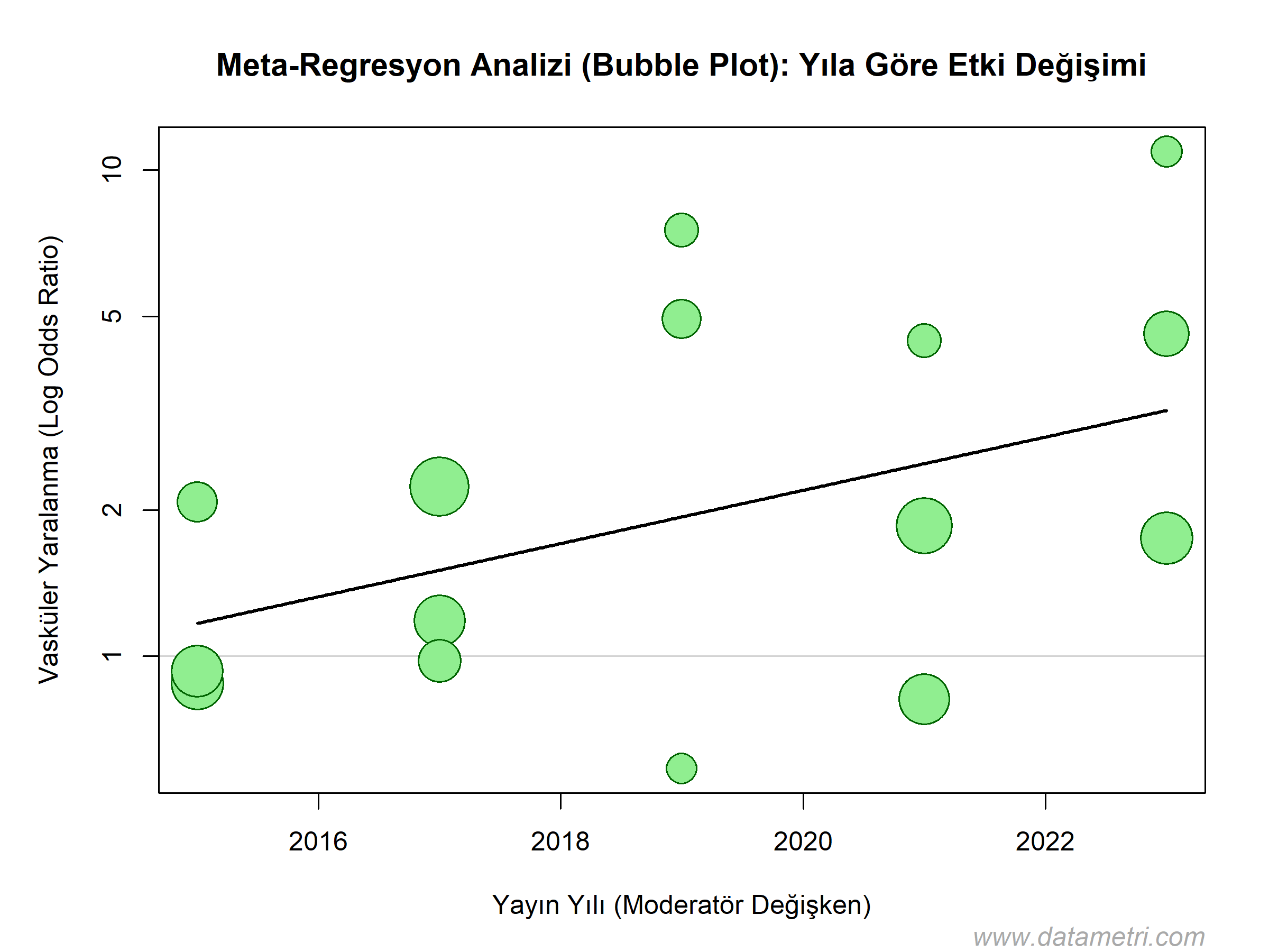
Meta-Regression: Is an advanced analysis model that tests how the effect size changes depending on a continuous variable (e.g., age, dose, publication year) rather than a categorical one.

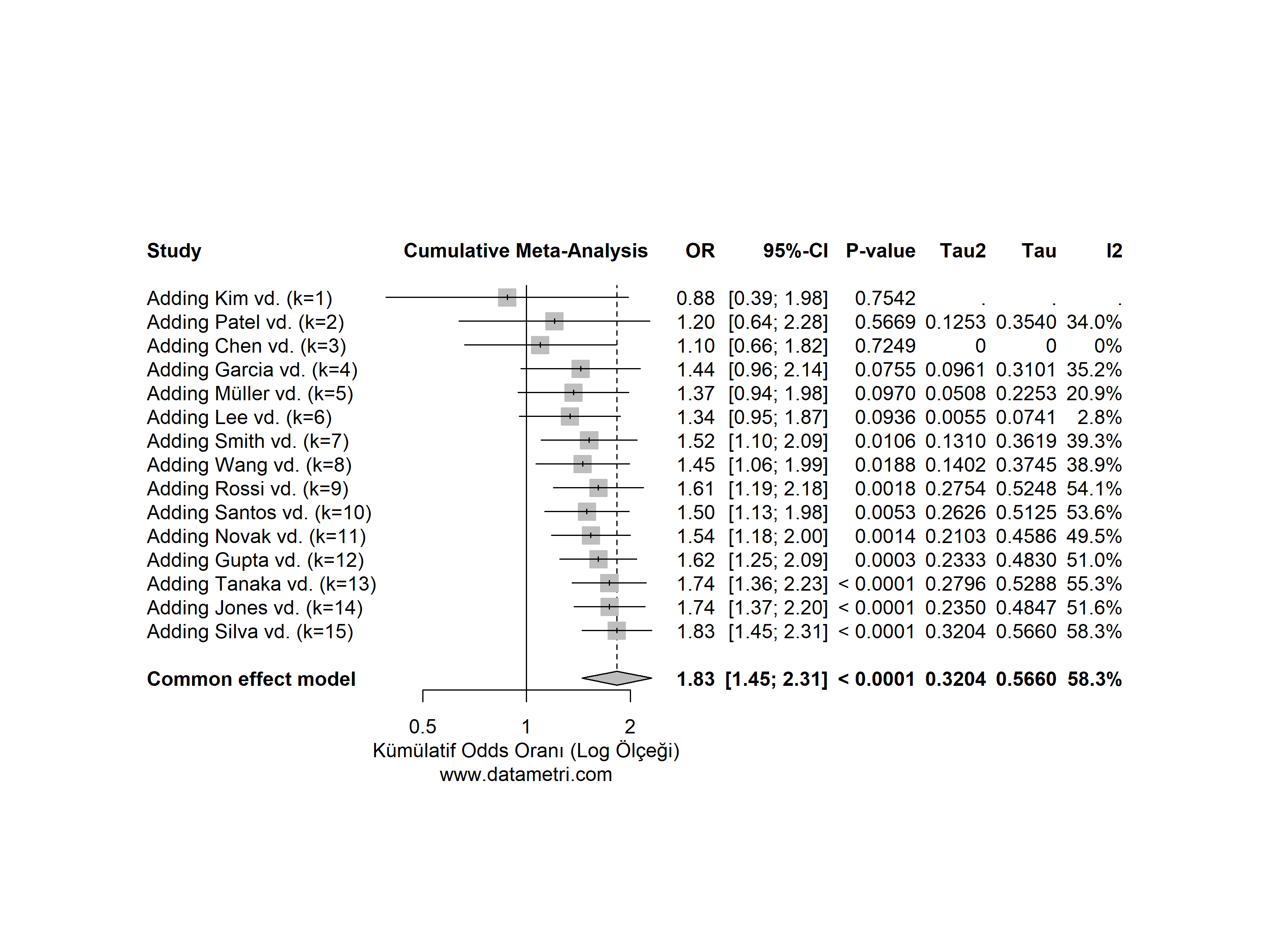
Cumulative Meta-Analysis: Puts an end to literature debates by presenting, from a historical perspective, when scientific evidence became "definitive" on the timeline.

Which Questions Does This Analysis Answer?
  • Does the effectiveness of the applied treatment systematically decrease as the mean age (continuous variable) of patients increases?
  • After the study conducted in which year did the evidence on a specific topic in the scientific world finally reach a point of statistical saturation?
Added Value to Your Research

Adds a causal depth to the meta-analysis. In research grant applications, it is a strategic necessity to prove to funding agencies (TÜBİTAK, NIH) the answer to the question, "Why do we need / not need to conduct this study?".

Meta-Regression Bubble Plot
Bubble Plot: Displays the relationship between effect size and a continuous moderator (e.g., publication year). The red regression line and its surrounding confidence interval denote the direction and trend of the moderating effect.
Cumulative Forest Plot
Cumulative Forest Plot: Incorporates studies into the model one by one, sorted by publication year. The narrowing of the diamond width (shrinking of the confidence interval) proves how prediction precision increases over time.
05
Multivariate Causal Networks (Structural Equation Modeling)
SEM / MSEM / RI-CLPM Causal Networks
▼

Modern scientific research has reached a complexity where multidimensional phenomena such as human behavior, clinical pathologies, or organizational dynamics can no longer be explained by one-way, linear, and isolated variable pairs. International peer-reviewed journals in the Q1 segment and top-tier funding boards (TÜBİTAK, NIH, Horizon Europe) now demand going beyond the shallow question of "Which variables are correlated with each other?".

A. Full Structural Equation Modeling (Full SEM): Mediation Mechanisms

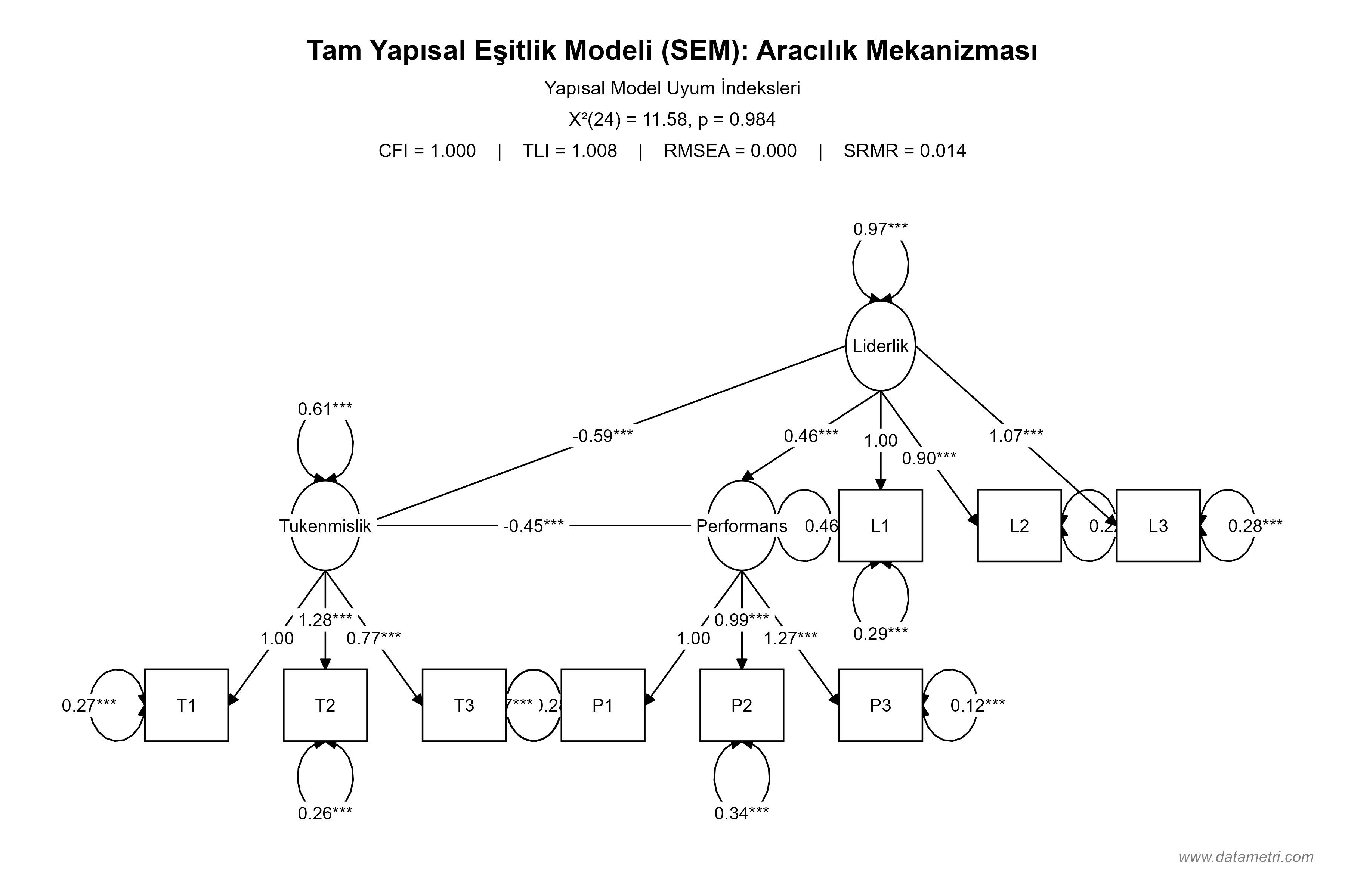
The traditional Baron and Kenny stepwise regression method resolves multiple paths independently of each other, increasing the Type I error rate. Datametri's Full Structural Model simultaneously resolves the entire causal network in a single variance-covariance matrix.

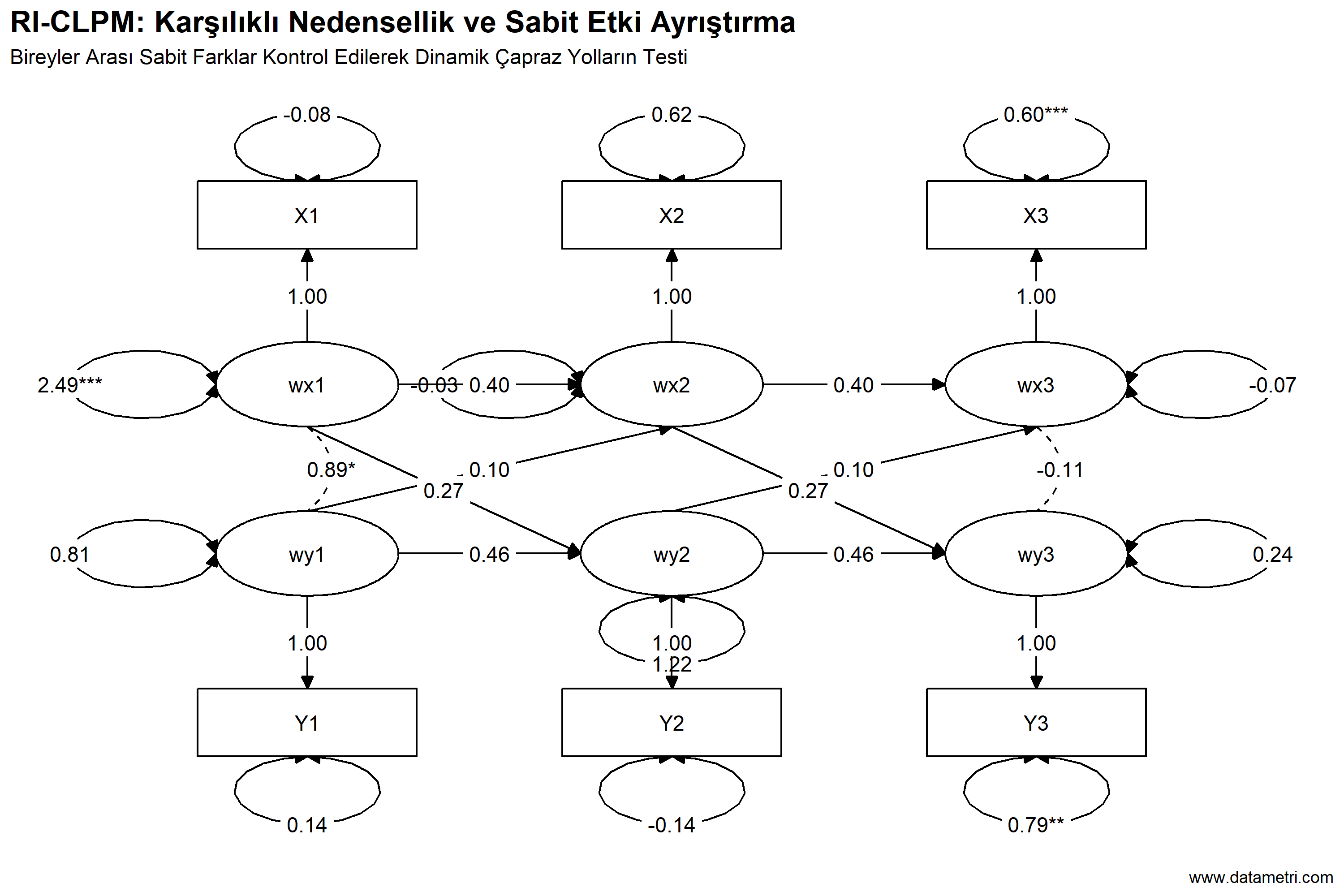
B. Multilevel SEM (MSEM) and RI-CLPM (Reciprocal Causality)

Applying standard regression to hierarchical data creates an "Ecological Fallacy." MSEM mathematically separates individual and group-level error margins. The RI-CLPM model, on the other hand, proves "Pure Causal Inference" by eliminating trait-like stable properties among individuals in longitudinal data.

Full Structural Equation Modeling and Mediation Effect
The statistical significance of the Mediation effect was tested with confidence intervals obtained by resampling the dataset thousands of times (Bootstrap resampling).
RI-CLPM Reciprocal Causality
The RI-CLPM diagram isolates individuals' invariant personality traits (Random Intercepts) in time series data and parameterizes the cross-lagged paths between variables in an error-free causality loop.
06
Network Meta-Analysis (Multiple-Treatment Comparison and Ranking)
Network Meta-Analysis P-score / SUCRA Node-Splitting
▼
"Compare Every Treatment at Once, Within a Single Evidence Network"

Conventional pairwise meta-analysis compares only two interventions. In clinical practice, however, decision-makers often have to choose among many options that have never been compared head-to-head. Network Meta-Analysis (NMA) combines direct (head-to-head) and indirect (via a common comparator) evidence in a single statistical model, comparing all treatments simultaneously and ranking them by efficacy.

Datametri's NMA workflow delivers, in a single protocol: a frequentist random-effects model (REML) that correctly handles the variance-covariance structure of multi-arm studies; multi-outcome (continuous and binary) analysis; global and local consistency tests; treatment ranking; sensitivity analyses; and evidence-certainty outputs (RoB 2 / GRADE-CINeMA). A Bayesian (gemtc) alternative can also be run on the same data.

All visuals in this section were generated from simulated (example) data to demonstrate the methodology; they do not represent a real clinical finding.

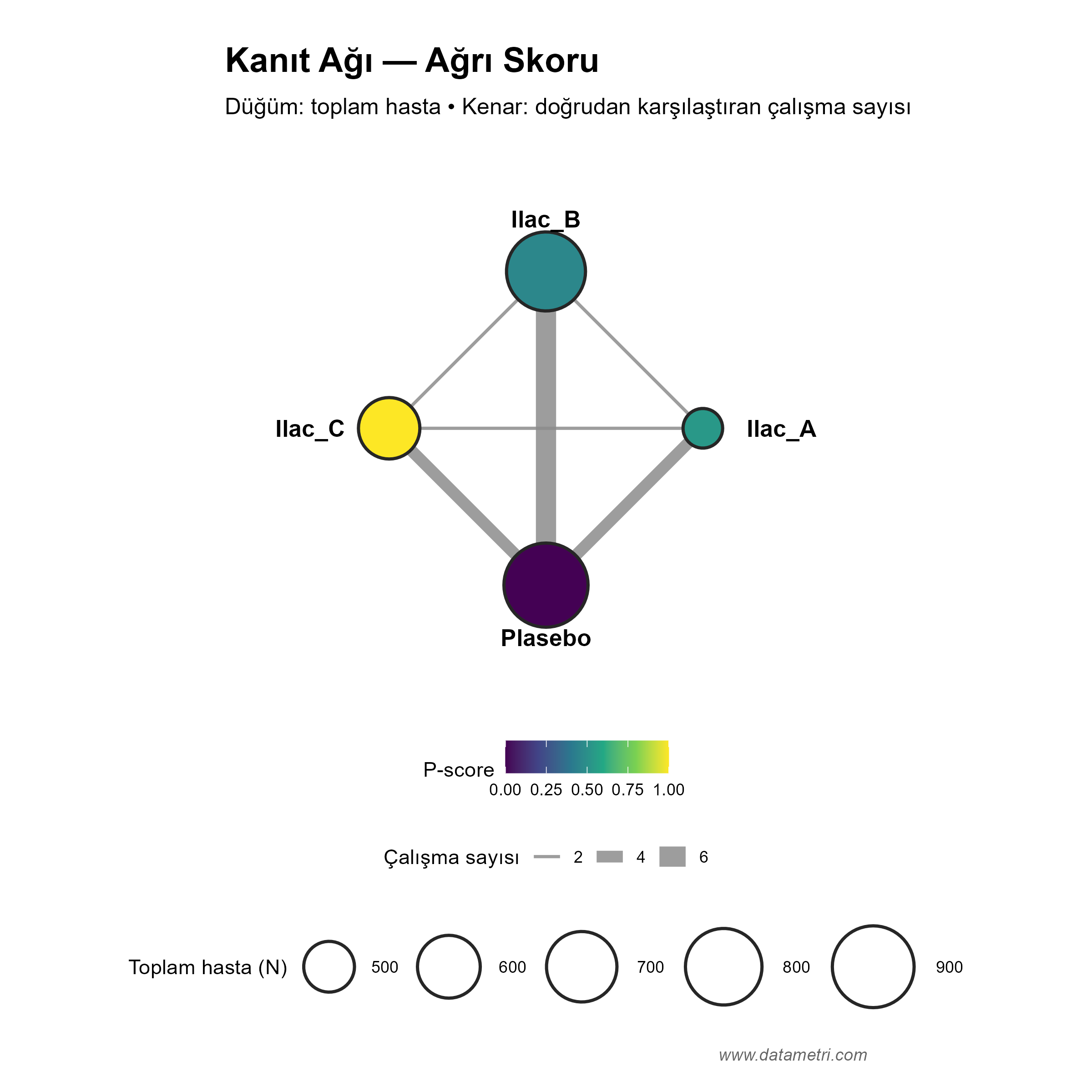
A. Evidence Network (Network Geometry)

The first step is to map which treatments have been compared directly, and in which studies. Closed loops in the network are where indirect evidence can be generated and consistency can be tested; in "star-shaped" networks connected only to a single reference (e.g., placebo), consistency cannot be assessed.

Which Questions Does This Analysis Answer?
  • What is the effect difference between treatments that have never been compared directly, and how precise is it?
  • Which treatment ranks best on the outcome of interest, and how reliable is that ranking?
  • Are direct and indirect evidence consistent with each other (transitivity / consistency assumption)?
Added Value to Your Research

Answers the question of "comparative effectiveness across all options", sought in clinical guidelines and health technology assessment (HTA), with a single model and transparent reporting. It also shows where the network is thin, documenting the need for future studies.

Network Meta-Analysis Evidence Network
Evidence Network Plot: Each node is a treatment; each edge represents studies that compare the two treatments directly. Node size shows total patients, edge thickness shows the number of studies, and node colour shows the ranking score (P-score).

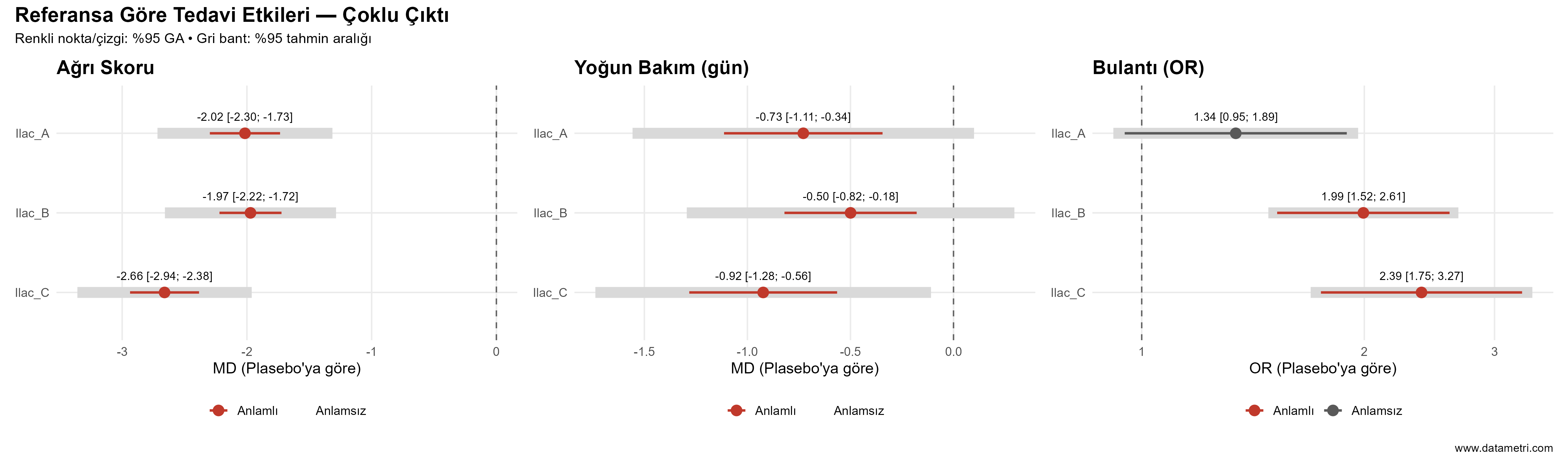
B. Multi-Outcome Effect Estimates

Each treatment's effect relative to the reference is estimated as a mean difference (MD) for continuous outcomes such as pain score and ICU stay, and as an odds ratio (OR) for binary outcomes such as nausea. Alongside confidence intervals, prediction intervals are reported, projecting heterogeneity onto the range of effects expected in a future study.

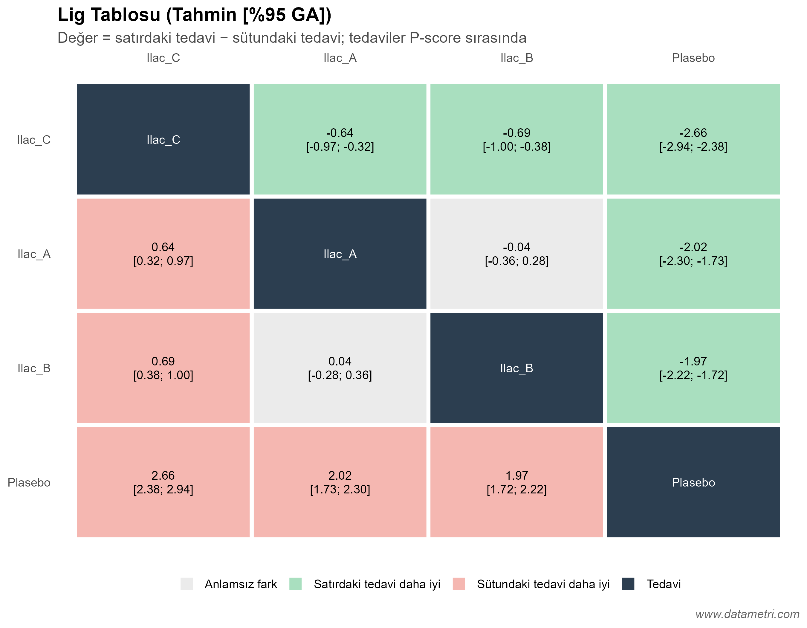
C. League Table

Comparative effects between all pairs of treatments are presented in a single matrix. Treatments are ordered by P-score, and colour coding shows at a glance whether a difference is statistically significant and which treatment it favours.

Multi-Outcome Network Meta-Analysis Forest Plot
Multi-Outcome Forest Plot: The point and line show the effect estimate versus the reference and its 95% confidence interval; the grey band behind shows the 95% prediction interval. An interval that does not cross the null line (0 for MD, 1 for OR) indicates a significant effect.
Network Meta-Analysis League Table Heatmap
League Table: Each cell gives the effect of the row treatment relative to the column treatment, with its confidence interval. Green cells show that the row treatment is significantly better, red cells that the column treatment is significantly better, and grey cells that there is no significant difference.

D. Treatment Ranking: P-score and SUCRA

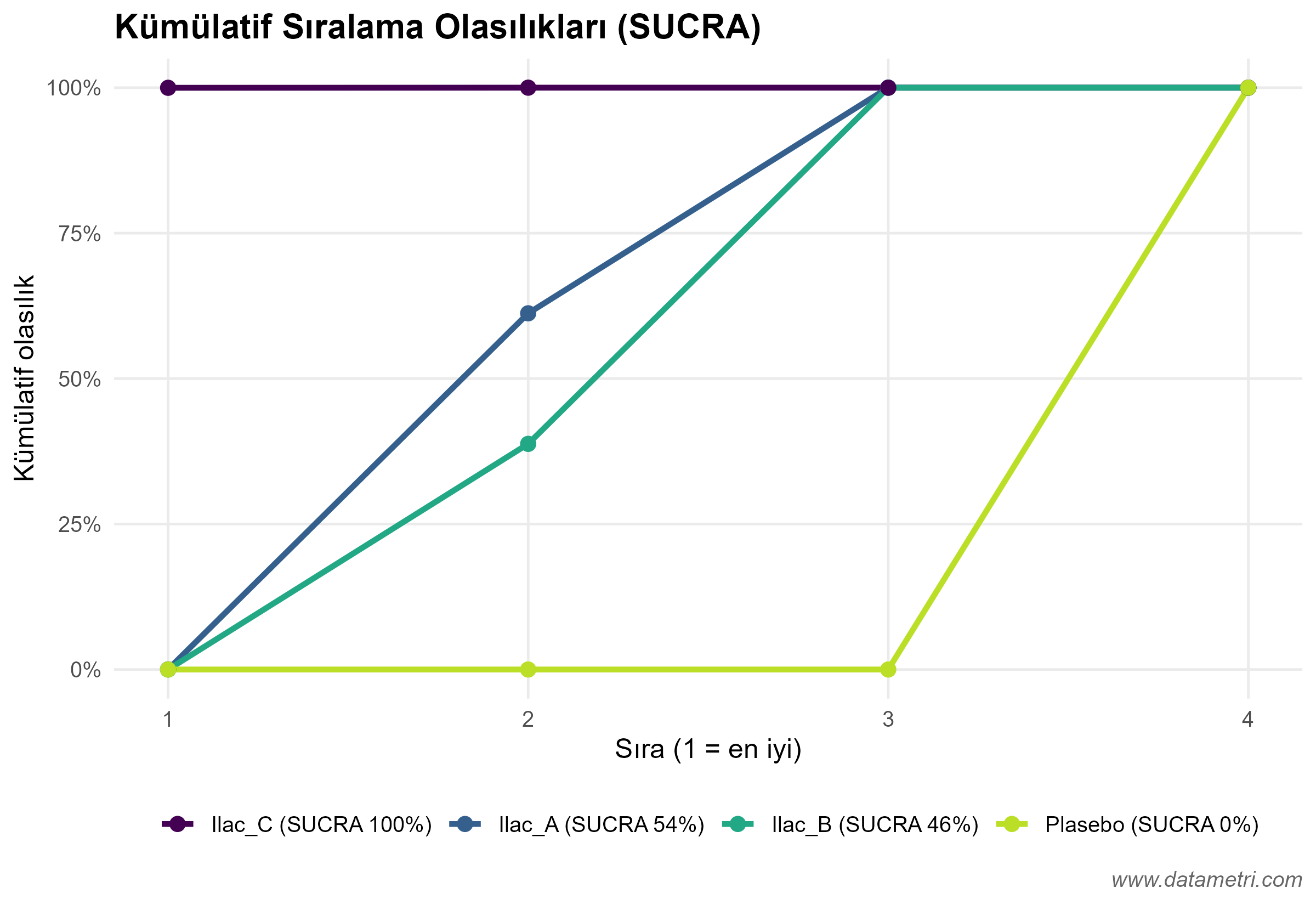
The P-score expresses the mean probability that a treatment is better than the others; SUCRA (Surface Under the Cumulative Ranking curve) is the area under the simulation-based cumulative ranking curve. The two measures are very close to each other; ranking is computed according to the direction of the outcome (whether lower or higher is better).

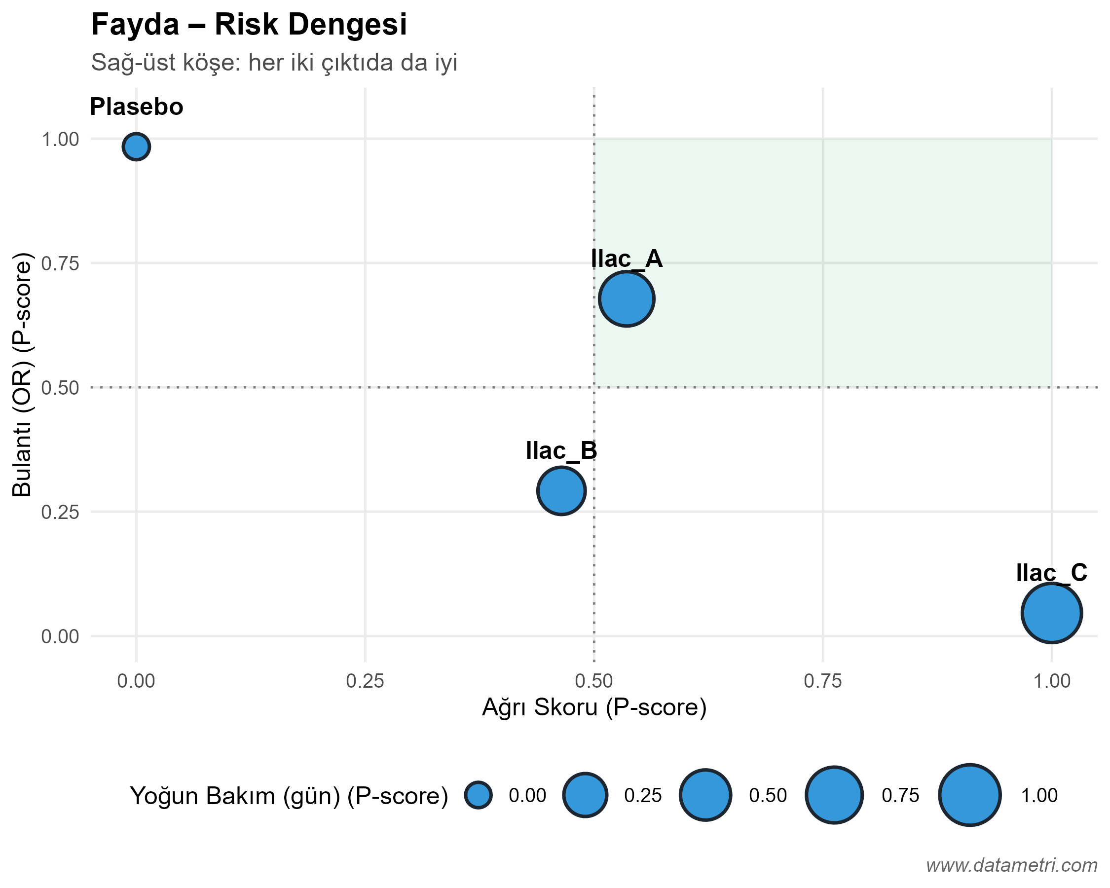
E. Benefit–Risk Balance

A treatment ranked best on one outcome may rank worst on a safety outcome. The multi-outcome heatmap and the two-outcome scatter plot make the trade-off between efficacy and safety visible. Rankings should be read only as a supporting summary, interpreted together with effect sizes and certainty of evidence.

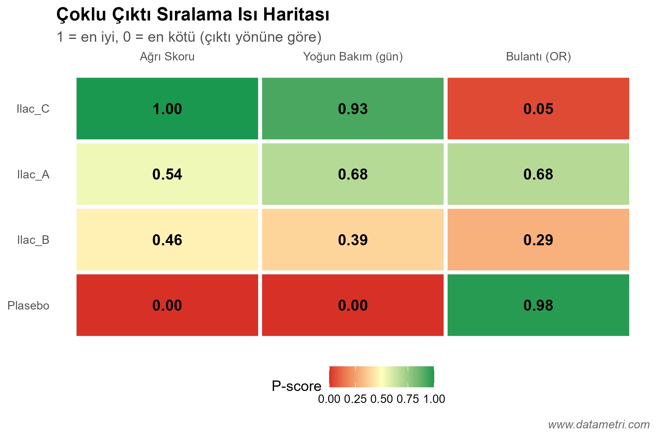
P-score Ranking Heatmap
Ranking Heatmap: Rows represent treatments and columns represent outcomes. Green cells show a high (good) P-score on that outcome, red cells a low (poor) P-score.
Benefit-Risk Scatter Plot
Benefit–Risk Plot: The axes are P-scores on two different outcomes. Treatments approaching the upper-right corner are advantageous on both outcomes; point size encodes a third outcome.
SUCRA Cumulative Ranking Curves
Cumulative Ranking Curves: The faster a curve rises, the higher the probability that the treatment ranks among the top positions. The area under each curve gives its SUCRA value; the percentages in the legend summarize the treatments.

F. Consistency and Heterogeneity Assessment

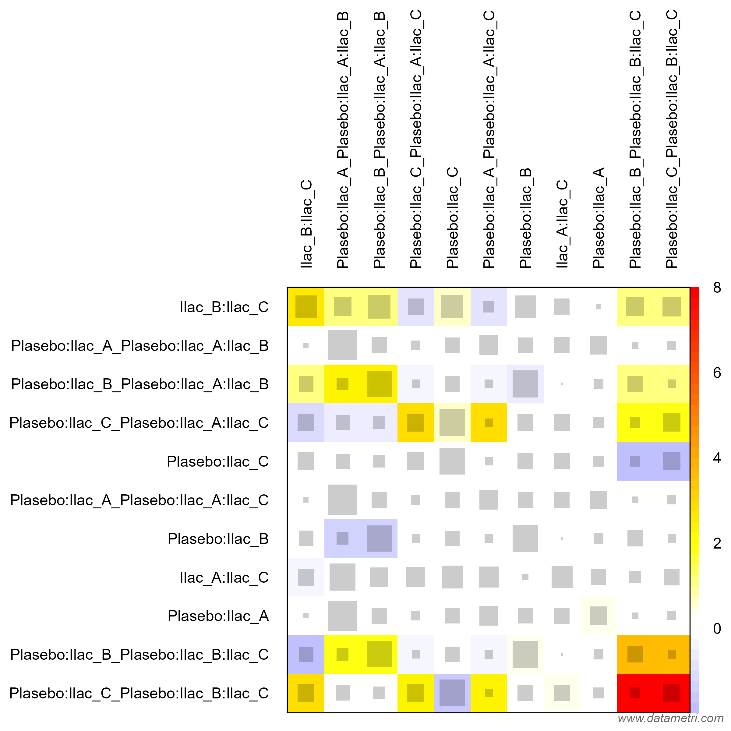
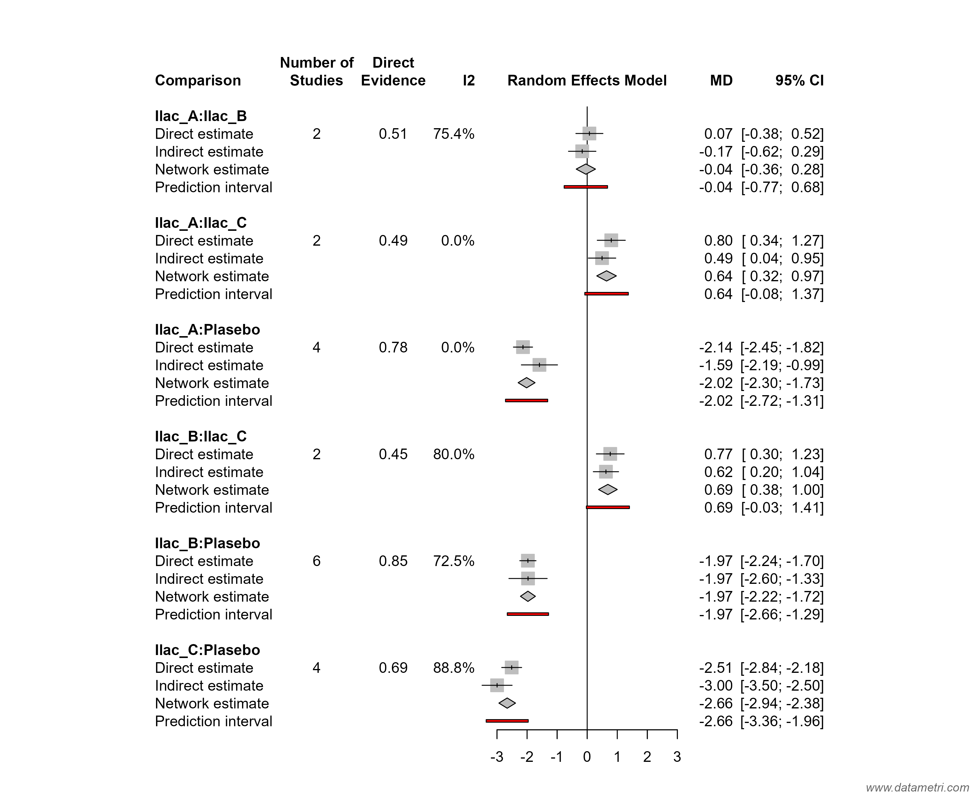
The validity of an NMA rests on the assumption that indirect evidence agrees with direct evidence. We test this assumption at three levels: (1) the design-by-treatment interaction test for global inconsistency, (2) the net-heat plot to locate sources of inconsistency, and (3) node-splitting, which separates direct and indirect estimates for each comparison. Network-level heterogeneity is tabulated with τ², I² and Q statistics.

G. Evidence Contribution Matrix

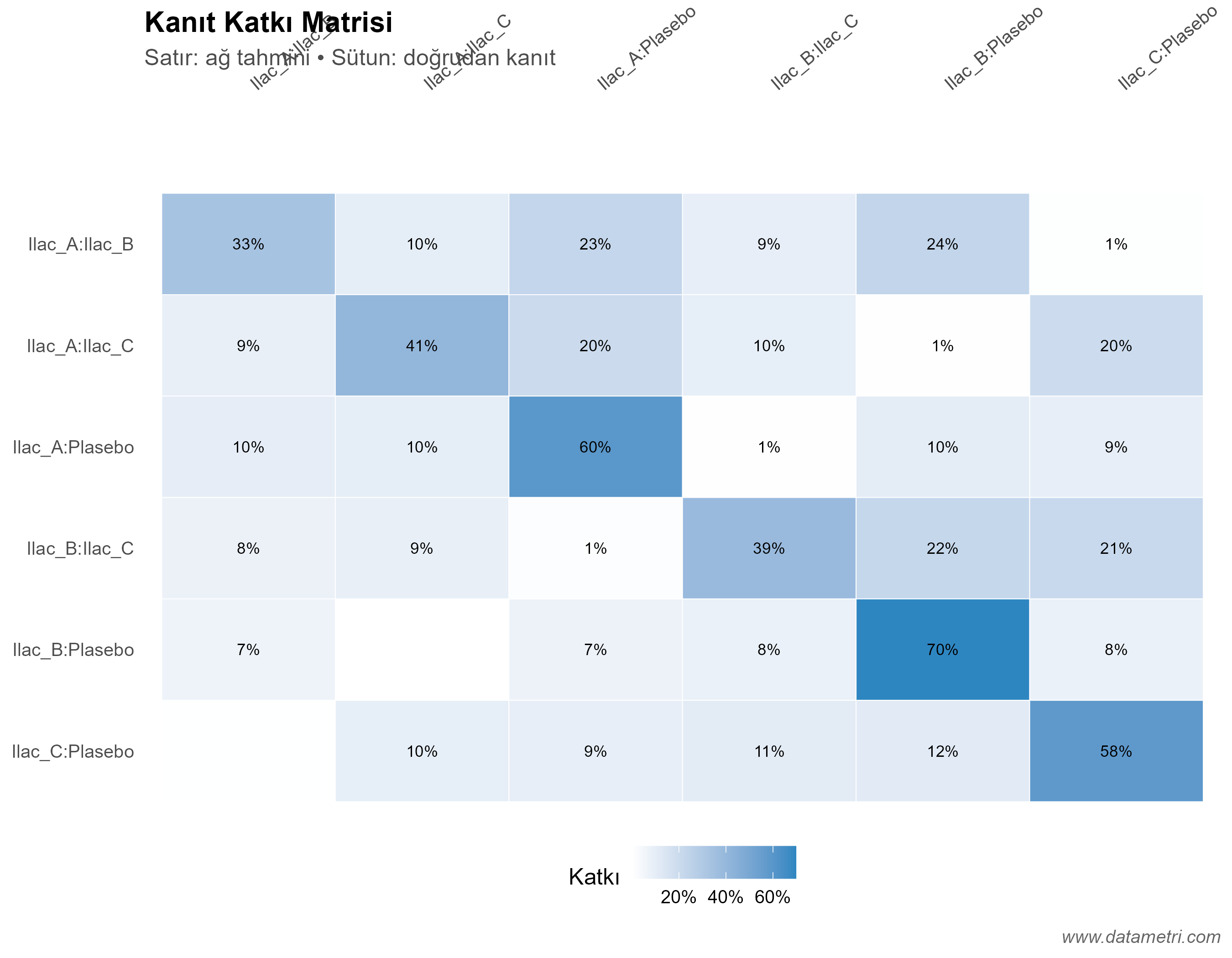
Shows which direct comparisons feed each network estimate, and in what proportion. This makes transparent the cases where a result rests on only a few small studies or on indirect evidence; this information is a direct input to certainty-of-evidence grading with GRADE/CINeMA.

Net Heat Plot Inconsistency Heatmap
Net-Heat Plot: Grey squares show the influence of a given design on the network estimate, while coloured areas show the inconsistency associated with that design. Dark blocks point to the comparisons that may be the source of inconsistency.
Node-Splitting Direct and Indirect Evidence Forest Plot
Node-Splitting: For each comparison, the direct, indirect and network (combined) estimates are shown side by side. A significant difference between direct and indirect estimates signals local inconsistency.
Evidence Contribution Matrix
Contribution Matrix: Rows show network estimates and columns show direct evidence. The percentage in a cell is the contribution of that direct evidence to the corresponding network estimate.

H. Risk of Bias (RoB 2) and Certainty of Evidence

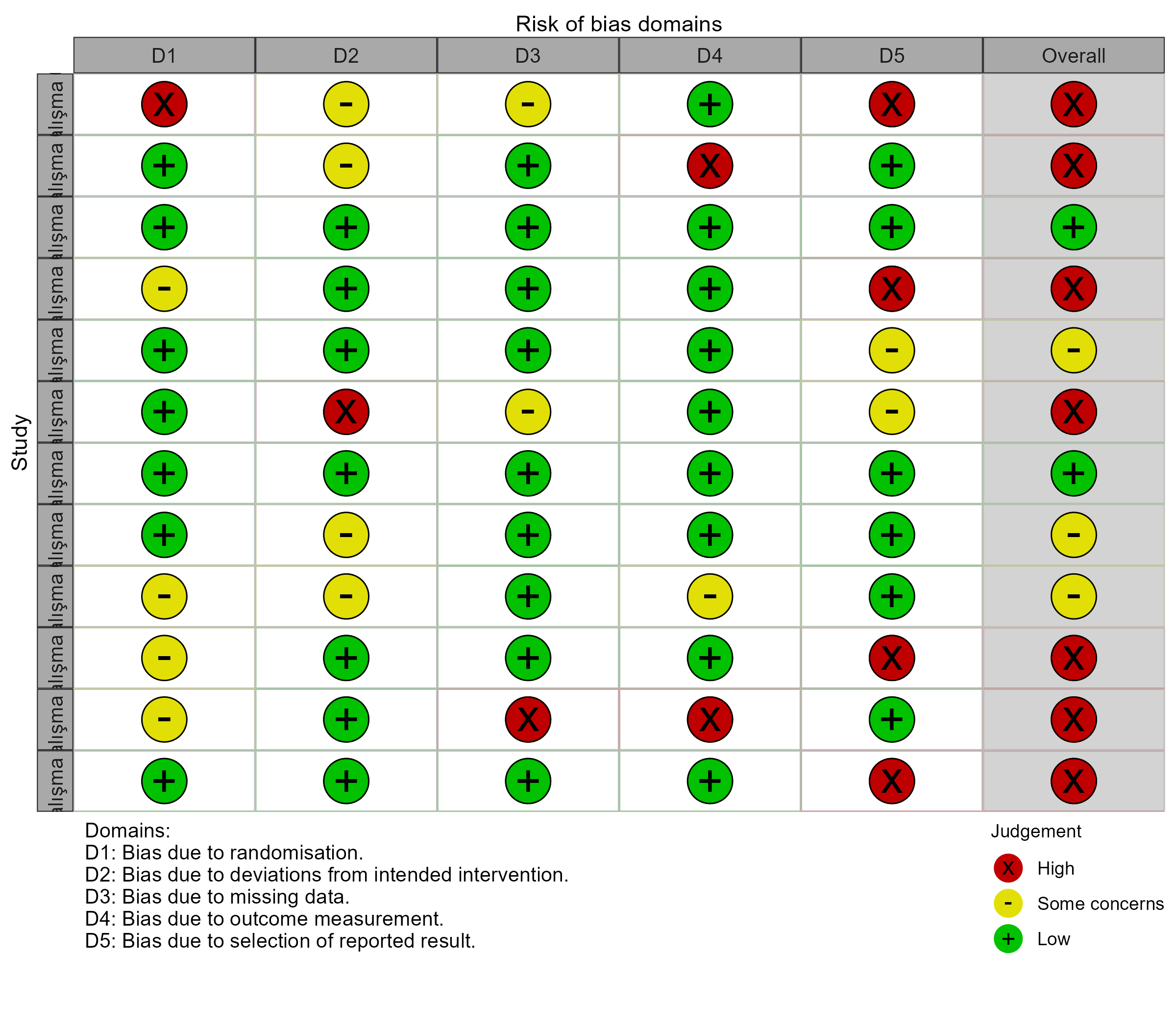
Every study is assessed across the RoB 2 domains (randomization, deviations, missing data, measurement, reporting), and traffic-light and summary plots are prepared. The same assessment is exported together with study-level data in the format expected by the CINeMA platform, making it ready for GRADE-based confidence rating of network estimates.

I. Small-Study Effects and Meta-Regression

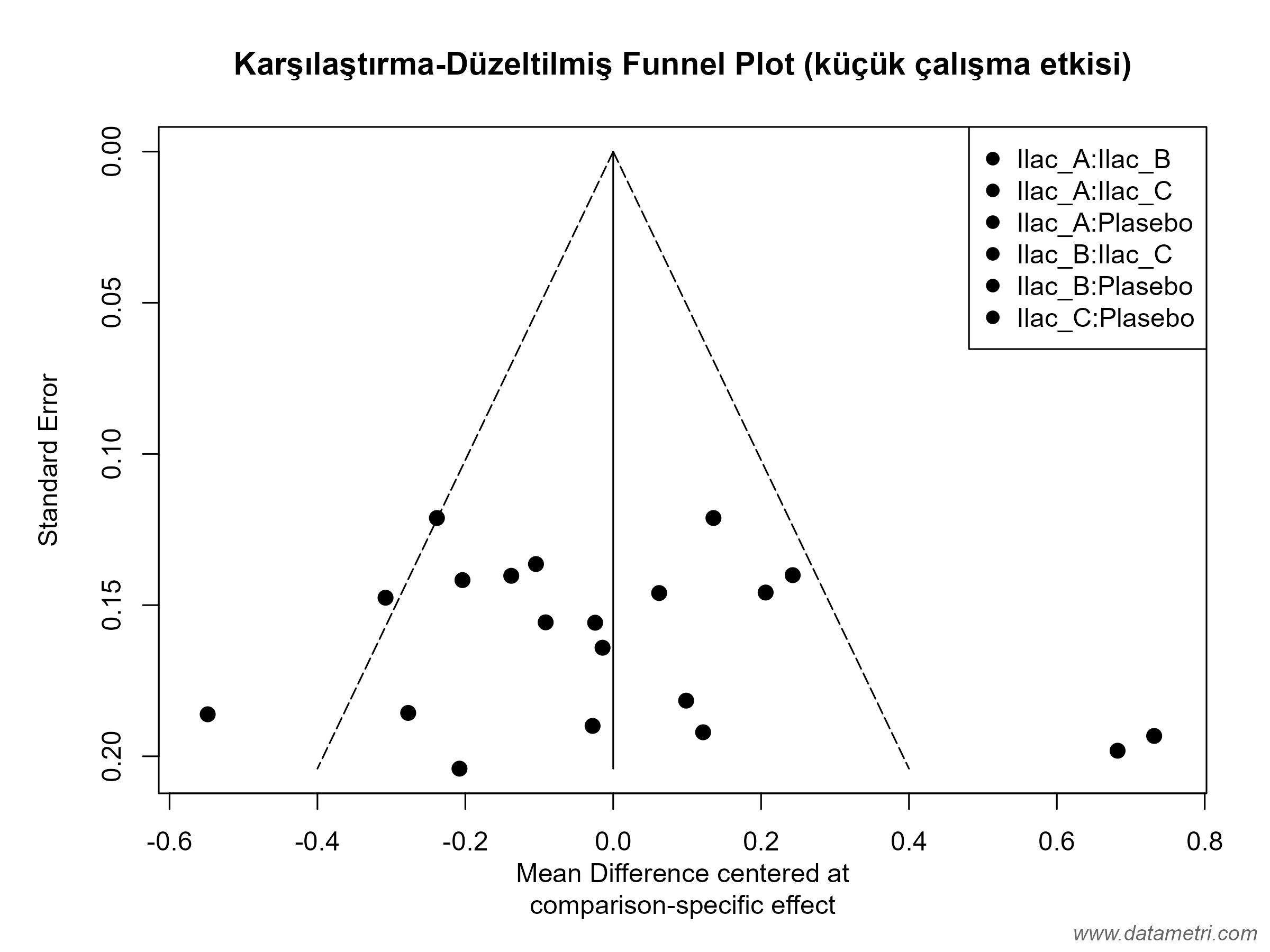
The comparison-adjusted funnel plot visualizes small-study effects and possible publication bias across the network. Network meta-regression is added for continuous moderators such as publication year. When the number of studies is small (e.g., < 10), the power of these tests is low, and interpretation is made with this limitation stated.

J. Sensitivity Analyses

Whether results depend on a single study or a modelling choice is tested through scenarios in which each study is excluded in turn (leave-one-out), studies at high risk of bias are removed, and a common-effect model is used.

Risk of Bias Traffic Light Plot
RoB 2 Traffic Light Plot: Green indicates low, yellow some concerns, and red high risk of bias. The last column gives the overall risk-of-bias judgement for the study.
Comparison-Adjusted Funnel Plot
Comparison-Adjusted Funnel Plot: Points show each study's deviation from the pooled estimate of its comparison. A distribution symmetric around zero suggests no small-study effects; asymmetry may be a signal of bias.
Leave-One-Out Sensitivity Analysis
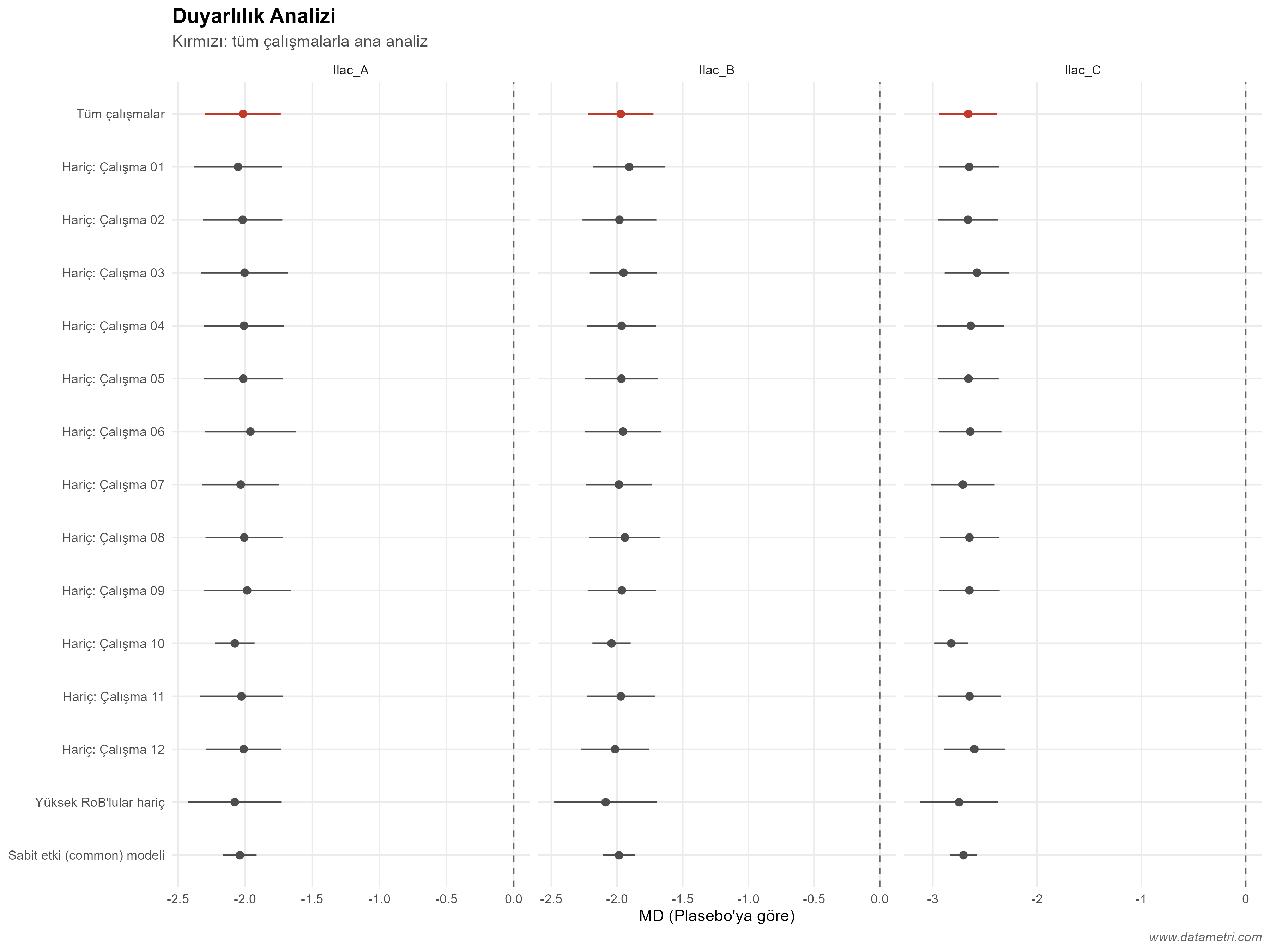
Sensitivity Plot: Each panel shows one treatment; the red point is the main analysis with all studies. If the estimate and its interval remain largely unchanged across the other scenarios, the result is robust.

Let's Transform Literature into a Scientific Evidence Set

Share the quantitative studies you've compiled and your analysis protocol with us; let's collaboratively prepare your research into a high-impact Meta-Analysis article compliant with PRISMA standards.